1.11 Spatial Data in R

1.11.1 Background

In ecological and geographical research, it is common to work with data that has a spatial component—that is, data associated with a specific location on Earth. For example, we might study the elevation of a forest plot, the location of a species observation, or the climate of a region. These types of data are known as spatial data, and they allow us to connect real-world phenomena with their geographic position.

Spatial data is the foundation of Geographic Information Systems (GIS), which are tools used to store, analyze, and visualize geographical information. While many researchers use GIS software such as QGIS or ArcGIS, R also offers powerful tools for handling spatial data, especially for analysis and automation.

There are two main formats of spatial data:

Vector data, which represents discrete objects like points (e.g., species occurrences), lines (e.g., roads), or polygons (e.g., country borders).
Raster data, which represents continuous surfaces such as temperature, elevation, or land cover, typically stored in a regular grid of pixels.

In this lesson, we introduce two R packages widely used to work with spatial data:

sf (Simple Features): for vector data
terra: for raster data

The goal is to explore the basic structure of spatial objects and understand how to interact with them in R. This will prepare you for more advanced operations like mapping, which we will cover in the next lesson.

1.11.2 Learning objectives

By the end of this lesson, you will be able to:

Recognize and describe vector and raster data structures in R.
Use sf and terra to load, explore, and filter spatial data.
Understand basic spatial metadata: CRS, resolution, and extent.
Export spatial objects to common GIS file formats.

1.11.3 Contents

This session introduces the basic logic of working with spatial data in R. Important spatial concepts:

Geometry: The shape or location (e.g., a point or polygon).
Attributes: Descriptive data linked to each feature (e.g., country name, elevation).
CRS (Coordinate Reference System): Tells R how to interpret the coordinates (e.g., in meters or degrees).
Raster resolution: The size of each pixel in a raster layer.

This session focuses on exploring data, not creating maps. The next lesson will cover visualization.

1.11.4 Literature

Geocomputation with R, Chapters 2, 4 & 6. https://r.geocompx.org/

1.11.5 Necessary preparation

You do not need any previous experience with R or GIS.

1.11.6 Tutorial: Exploring spatial data with `sf` and `terra`

1.11.6.1 Loading libraries

Before you begin, make sure you have the sf package installed. You can install it with the following command:

install.packages("sf")
install.packages("terra")

library(sf)

## Warning: Paket 'sf' wurde unter R Version 4.4.3 erstellt

## Linking to GEOS 3.13.0, GDAL 3.10.1, PROJ 9.5.1; sf_use_s2() is TRUE

library(terra)

## Warning: Paket 'terra' wurde unter R Version 4.4.3 erstellt

## terra 1.8.54

## 
## Attache Paket: 'terra'

## Das folgende Objekt ist maskiert 'package:phytools':
## 
##     rescale

## Die folgenden Objekte sind maskiert von 'package:ape':
## 
##     rotate, trans, zoom

library(tidyverse)

## ── Attaching core tidyverse packages ────────────────────────── tidyverse 2.0.0 ──
## ✔ dplyr     1.1.4     ✔ readr     2.1.5
## ✔ forcats   1.0.0     ✔ stringr   1.5.1
## ✔ ggplot2   3.5.1     ✔ tibble    3.2.1
## ✔ lubridate 1.9.3     ✔ tidyr     1.3.1
## ✔ purrr     1.0.2

## ── Conflicts ──────────────────────────────────────────── tidyverse_conflicts() ──
## ✖ tidyr::extract() masks terra::extract()
## ✖ dplyr::filter()  masks stats::filter()
## ✖ dplyr::lag()     masks stats::lag()
## ✖ purrr::map()     masks maps::map()
## ✖ dplyr::where()   masks ape::where()
## ℹ Use the conflicted package (<http://conflicted.r-lib.org/>) to force all conflicts to become errors

1.11.6.2 Vector Data using Simple Feature Classes `sf`

The sf package in R is a powerful tool for working with spatial data. It provides a wide range of functions and methods for reading, writing, manipulating, and visualizing spatial data. In this tutorial, we will cover several essential aspects of working with the sf package:

1.11.6.3 Creating Simple Feature Geometry (SFG) Objects

Create points

# Create a simple feature geometry with 3 points
points <- st_sfc(
  st_point(c(0, 0)),
  st_point(c(1, 1)),
  st_point(c(2, 2))
)

# Display structure
points

## Geometry set for 3 features 
## Geometry type: POINT
## Dimension:     XY
## Bounding box:  xmin: 0 ymin: 0 xmax: 2 ymax: 2
## CRS:           NA

## POINT (0 0)

## POINT (1 1)

## POINT (2 2)

Create polygons

# Create two polygons and store as an SFC object
polygons <- st_sfc(
  st_polygon(list(rbind(c(0,0), c(0,1), c(1,1), c(1,0), c(0,0)))),
  st_polygon(list(rbind(c(1,1), c(1,2), c(2,2), c(2,1), c(1,1))))
)

# Display
polygons

## Geometry set for 2 features 
## Geometry type: POLYGON
## Dimension:     XY
## Bounding box:  xmin: 0 ymin: 0 xmax: 2 ymax: 2
## CRS:           NA

## POLYGON ((0 0, 0 1, 1 1, 1 0, 0 0))

## POLYGON ((1 1, 1 2, 2 2, 2 1, 1 1))

To create a multipoint object from scratch, we use the st_multipoint function.

# Erstellen eines Mehrpunktobjekts von Grund auf
multipoints <- st_multipoint(x = matrix(c(0, 0), c(1, 1), c(2, 2)))

# Drucken des Mehrpunktobjekts
multipoints

## MULTIPOINT ((0 0))

1.11.6.4 Creating a Multi-Point Object from a .csv File

You can also create multipoint objects from CSV data. First, load a CSV file with spatial coordinates. You can find the sample data on ILIAS. Remember to specify your working directory and the correct path.

library(readr)
# Load data from a CSV file
data <- read_csv("data/iNaturalist.csv")

# Convert to sf object using longitude and latitude columns
multipoints_from_csv <- st_as_sf(data, coords = c("longitude", "latitude"), crs = 4326)

# Inspect object
head(multipoints_from_csv)

1.11.6.5 Creating multi-polygon objects from a shapefile

You can create a multi-polygon object from a shapefile using the st_read function; for example, use the Level 3 Botanical Lands, which you must first unpack.

# Read a shapefile (e.g., botanical boundaries)
polygons_from_shapefile <- st_read("data/bot_count.shp")

## Reading layer `bot_count' from data source 
##   `C:\Users\zizka_lokal\Dropbox\01_projects\00_bsc_AM_biodiv_pflanzen_2025\Übung\bsc-biodiv-der-pflanzen\data\bot_count.shp' 
##   using driver `ESRI Shapefile'
## Simple feature collection with 369 features and 4 fields
## Geometry type: MULTIPOLYGON
## Dimension:     XY
## Bounding box:  xmin: -180 ymin: -90 xmax: 179.9999 ymax: 83.62361
## Geodetic CRS:  WGS 84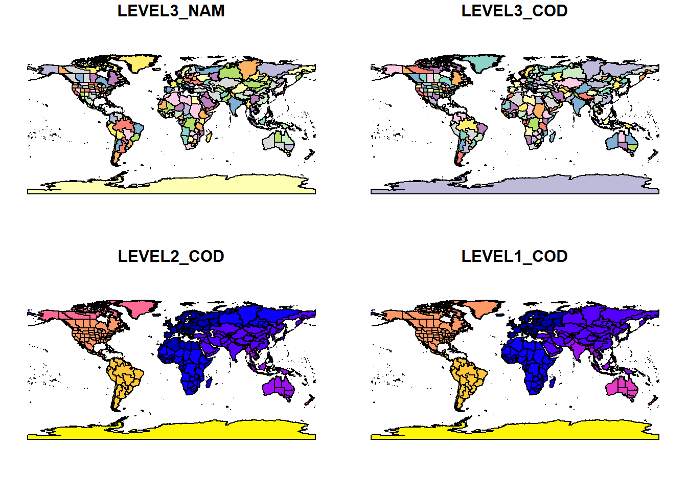

# Quick preview
plot(polygons_from_shapefile)

1.11.6.6 Filtering and selecting attributes

You can filter and summarize data based on attributes by using the dplyr package in combination with the sf package.

# Filter polygons with LEVEL1_COD equal to 7
filtered_polygons <- polygons_from_shapefile %>%
  filter(LEVEL1_COD == 7)

# Filter where LEVEL1_COD > 5
filtered_polygons <- polygons_from_shapefile %>%
  filter(LEVEL1_COD > 5)

# Select specific attribute columns
selected_attributes <- polygons_from_shapefile %>%
  select(LEVEL3_COD, LEVEL3_NAM)

# Display result
head(selected_attributes)

## Simple feature collection with 6 features and 2 fields
## Geometry type: MULTIPOLYGON
## Dimension:     XY
## Bounding box:  xmin: -120.0014 ymin: -55.05169 xmax: 74.91577 ymax: 60
## Geodetic CRS:  WGS 84
##   LEVEL3_COD          LEVEL3_NAM                       geometry
## 1        ABT             Alberta MULTIPOLYGON (((-114.8308 5...
## 2        AFG         Afghanistan MULTIPOLYGON (((71.24197 38...
## 3        AGE Argentina Northeast MULTIPOLYGON (((-61.86666 -...
## 4        AGS     Argentina South MULTIPOLYGON (((-68.59916 -...
## 5        AGW Argentina Northwest MULTIPOLYGON (((-65.75386 -...
## 6        ALA             Alabama MULTIPOLYGON (((-88.16472 3...

1.11.6.7 Saving spatial data to disk

# Save spatial object to a new shapefile
st_write(polygons_from_shapefile, "data/test_shapefile.shp", delete_layer = TRUE)

## Deleting layer `test_shapefile' using driver `ESRI Shapefile'
## Writing layer `test_shapefile' to data source 
##   `data/test_shapefile.shp' using driver `ESRI Shapefile'
## Writing 369 features with 4 fields and geometry type Multi Polygon.

1.11.7 Optional: Spatial data tutorial

1.11.7.1 Exploring built-in `sf` data

We’ll use a built-in dataset that comes with the sf package:

# Example vector data: country polygons
world <- st_read(system.file("shape/nc.shp", package = "sf"))

## Reading layer `nc' from data source 
##   `C:\Users\zizka_lokal\AppData\Local\Programs\R\R-4.4.2\library\sf\shape\nc.shp' 
##   using driver `ESRI Shapefile'
## Simple feature collection with 100 features and 14 fields
## Geometry type: MULTIPOLYGON
## Dimension:     XY
## Bounding box:  xmin: -84.32385 ymin: 33.88199 xmax: -75.45698 ymax: 36.58965
## Geodetic CRS:  NAD27

# Explore structure
class(world)

## [1] "sf"         "data.frame"

head(world)

## Simple feature collection with 6 features and 14 fields
## Geometry type: MULTIPOLYGON
## Dimension:     XY
## Bounding box:  xmin: -81.74107 ymin: 36.07282 xmax: -75.77316 ymax: 36.58965
## Geodetic CRS:  NAD27
##    AREA PERIMETER CNTY_ CNTY_ID        NAME  FIPS FIPSNO CRESS_ID BIR74 SID74
## 1 0.114     1.442  1825    1825        Ashe 37009  37009        5  1091     1
## 2 0.061     1.231  1827    1827   Alleghany 37005  37005        3   487     0
## 3 0.143     1.630  1828    1828       Surry 37171  37171       86  3188     5
## 4 0.070     2.968  1831    1831   Currituck 37053  37053       27   508     1
## 5 0.153     2.206  1832    1832 Northampton 37131  37131       66  1421     9
## 6 0.097     1.670  1833    1833    Hertford 37091  37091       46  1452     7
##   NWBIR74 BIR79 SID79 NWBIR79                       geometry
## 1      10  1364     0      19 MULTIPOLYGON (((-81.47276 3...
## 2      10   542     3      12 MULTIPOLYGON (((-81.23989 3...
## 3     208  3616     6     260 MULTIPOLYGON (((-80.45634 3...
## 4     123   830     2     145 MULTIPOLYGON (((-76.00897 3...
## 5    1066  1606     3    1197 MULTIPOLYGON (((-77.21767 3...
## 6     954  1838     5    1237 MULTIPOLYGON (((-76.74506 3...

summary(world)

##       AREA          PERIMETER         CNTY_         CNTY_ID    
##  Min.   :0.0420   Min.   :0.999   Min.   :1825   Min.   :1825  
##  1st Qu.:0.0910   1st Qu.:1.324   1st Qu.:1902   1st Qu.:1902  
##  Median :0.1205   Median :1.609   Median :1982   Median :1982  
##  Mean   :0.1263   Mean   :1.673   Mean   :1986   Mean   :1986  
##  3rd Qu.:0.1542   3rd Qu.:1.859   3rd Qu.:2067   3rd Qu.:2067  
##  Max.   :0.2410   Max.   :3.640   Max.   :2241   Max.   :2241  
##      NAME               FIPS               FIPSNO         CRESS_ID     
##  Length:100         Length:100         Min.   :37001   Min.   :  1.00  
##  Class :character   Class :character   1st Qu.:37051   1st Qu.: 25.75  
##  Mode  :character   Mode  :character   Median :37100   Median : 50.50  
##                                        Mean   :37100   Mean   : 50.50  
##                                        3rd Qu.:37150   3rd Qu.: 75.25  
##                                        Max.   :37199   Max.   :100.00  
##      BIR74           SID74          NWBIR74           BIR79      
##  Min.   :  248   Min.   : 0.00   Min.   :   1.0   Min.   :  319  
##  1st Qu.: 1077   1st Qu.: 2.00   1st Qu.: 190.0   1st Qu.: 1336  
##  Median : 2180   Median : 4.00   Median : 697.5   Median : 2636  
##  Mean   : 3300   Mean   : 6.67   Mean   :1050.8   Mean   : 4224  
##  3rd Qu.: 3936   3rd Qu.: 8.25   3rd Qu.:1168.5   3rd Qu.: 4889  
##  Max.   :21588   Max.   :44.00   Max.   :8027.0   Max.   :30757  
##      SID79          NWBIR79                 geometry  
##  Min.   : 0.00   Min.   :    3.0   MULTIPOLYGON :100  
##  1st Qu.: 2.00   1st Qu.:  250.5   epsg:4267    :  0  
##  Median : 5.00   Median :  874.5   +proj=long...:  0  
##  Mean   : 8.36   Mean   : 1352.8                      
##  3rd Qu.:10.25   3rd Qu.: 1406.8                      
##  Max.   :57.00   Max.   :11631.0

# Plot geometry only
plot(st_geometry(world))

1.11.7.2 Accessing spatial metadata

# Coordinate Reference System
st_crs(world)

## Coordinate Reference System:
##   User input: NAD27 
##   wkt:
## GEOGCRS["NAD27",
##     DATUM["North American Datum 1927",
##         ELLIPSOID["Clarke 1866",6378206.4,294.978698213898,
##             LENGTHUNIT["metre",1]]],
##     PRIMEM["Greenwich",0,
##         ANGLEUNIT["degree",0.0174532925199433]],
##     CS[ellipsoidal,2],
##         AXIS["latitude",north,
##             ORDER[1],
##             ANGLEUNIT["degree",0.0174532925199433]],
##         AXIS["longitude",east,
##             ORDER[2],
##             ANGLEUNIT["degree",0.0174532925199433]],
##     ID["EPSG",4267]]

# View attribute names
names(world)

##  [1] "AREA"      "PERIMETER" "CNTY_"     "CNTY_ID"   "NAME"      "FIPS"     
##  [7] "FIPSNO"    "CRESS_ID"  "BIR74"     "SID74"     "NWBIR74"   "BIR79"    
## [13] "SID79"     "NWBIR79"   "geometry"

# Subset example
subset_world <- world[1:5, c("NAME", "AREA")]

# Export (optional)
st_write(subset_world, "data/subset_world.shp", delete_layer = TRUE)

## Deleting layer `subset_world' using driver `ESRI Shapefile'
## Writing layer `subset_world' to data source 
##   `data/subset_world.shp' using driver `ESRI Shapefile'
## Writing 5 features with 2 fields and geometry type Multi Polygon.

1.11.7.3 Working with raster data using `terra`

Now let’s look at raster data:

# Load package
library(terra)

# Create dummy raster
r <- rast(nrows = 10, ncols = 10, vals = 1:100)

# Display raster
plot(r)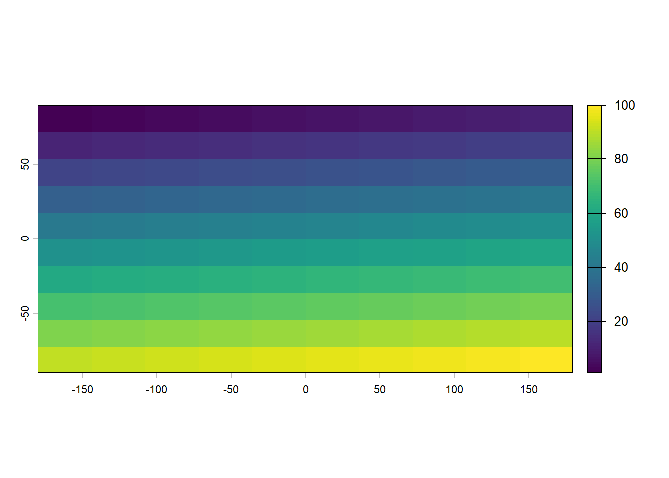

# Check properties
r

## class       : SpatRaster 
## size        : 10, 10, 1  (nrow, ncol, nlyr)
## resolution  : 36, 18  (x, y)
## extent      : -180, 180, -90, 90  (xmin, xmax, ymin, ymax)
## coord. ref. : lon/lat WGS 84 (CRS84) (OGC:CRS84) 
## source(s)   : memory
## name        : lyr.1 
## min value   :     1 
## max value   :   100

res(r)  # resolution

## [1] 36 18

ext(r)  # extent

## SpatExtent : -180, 180, -90, 90 (xmin, xmax, ymin, ymax)

crs(r)  # CRS (empty unless defined)

## [1] "GEOGCRS[\"WGS 84 (CRS84)\",\n    DATUM[\"World Geodetic System 1984\",\n        ELLIPSOID[\"WGS 84\",6378137,298.257223563,\n            LENGTHUNIT[\"metre\",1]]],\n    PRIMEM[\"Greenwich\",0,\n        ANGLEUNIT[\"degree\",0.0174532925199433]],\n    CS[ellipsoidal,2],\n        AXIS[\"geodetic longitude (Lon)\",east,\n            ORDER[1],\n            ANGLEUNIT[\"degree\",0.0174532925199433]],\n        AXIS[\"geodetic latitude (Lat)\",north,\n            ORDER[2],\n            ANGLEUNIT[\"degree\",0.0174532925199433]],\n    USAGE[\n        SCOPE[\"unknown\"],\n        AREA[\"World\"],\n        BBOX[-90,-180,90,180]],\n    ID[\"OGC\",\"CRS84\"]]"

1.11.7.4 Basic raster operations

# Access values
values(r)

##        lyr.1
##   [1,]     1
##   [2,]     2
##   [3,]     3
##   [4,]     4
##   [5,]     5
##   [6,]     6
##   [7,]     7
##   [8,]     8
##   [9,]     9
##  [10,]    10
##  [11,]    11
##  [12,]    12
##  [13,]    13
##  [14,]    14
##  [15,]    15
##  [16,]    16
##  [17,]    17
##  [18,]    18
##  [19,]    19
##  [20,]    20
##  [21,]    21
##  [22,]    22
##  [23,]    23
##  [24,]    24
##  [25,]    25
##  [26,]    26
##  [27,]    27
##  [28,]    28
##  [29,]    29
##  [30,]    30
##  [31,]    31
##  [32,]    32
##  [33,]    33
##  [34,]    34
##  [35,]    35
##  [36,]    36
##  [37,]    37
##  [38,]    38
##  [39,]    39
##  [40,]    40
##  [41,]    41
##  [42,]    42
##  [43,]    43
##  [44,]    44
##  [45,]    45
##  [46,]    46
##  [47,]    47
##  [48,]    48
##  [49,]    49
##  [50,]    50
##  [51,]    51
##  [52,]    52
##  [53,]    53
##  [54,]    54
##  [55,]    55
##  [56,]    56
##  [57,]    57
##  [58,]    58
##  [59,]    59
##  [60,]    60
##  [61,]    61
##  [62,]    62
##  [63,]    63
##  [64,]    64
##  [65,]    65
##  [66,]    66
##  [67,]    67
##  [68,]    68
##  [69,]    69
##  [70,]    70
##  [71,]    71
##  [72,]    72
##  [73,]    73
##  [74,]    74
##  [75,]    75
##  [76,]    76
##  [77,]    77
##  [78,]    78
##  [79,]    79
##  [80,]    80
##  [81,]    81
##  [82,]    82
##  [83,]    83
##  [84,]    84
##  [85,]    85
##  [86,]    86
##  [87,]    87
##  [88,]    88
##  [89,]    89
##  [90,]    90
##  [91,]    91
##  [92,]    92
##  [93,]    93
##  [94,]    94
##  [95,]    95
##  [96,]    96
##  [97,]    97
##  [98,]    98
##  [99,]    99
## [100,]   100

# Crop raster to specific extent
cropped <- crop(r, ext(1, 5, 1, 5))

# Save cropped raster
writeRaster(cropped, "data/cropped_raster.tif", overwrite = TRUE)

1.11.8 Tasks

Write an introductory paragraph explaining the difference between vector and raster data. Mention at least two examples of each in ecological research.
Use the st_read() function to load a shapefile of your choice (you can use bot_count.shp from class or one from a public source). Filter the dataset to show only a specific region, and save the filtered object as a new shapefile.
Create a raster object using the rast() function and populate it with random values. Crop the raster using a spatial extent and plot the result. What happens when you change the resolution?
Extract the CRS, extent, and resolution of both a vector and raster object. Compare them. What does this information tell you, and why is it important?