2.8 Spatial data and maps in R
2.8.1 Background
In ecological and geographical research, it is common to work with data that has a spatial component: data associated with a specific location on Earth. For example, we might study the elevation of a forest plot, the climate of a region, the area of a protected area, or the biome in which a plant was collected. These types of data are known as spatial data, and they connect real-world observations with geographic position.
Spatial data are the foundation of Geographic Information Systems (GIS): systems used to store, analyze, and visualize geographical information. Many researchers use GIS software such as QGIS or ArcGIS, but R also provides powerful tools for spatial analysis. The advantage of using R is that spatial operations can be integrated directly into reproducible workflows: data cleaning, statistics, mapping, and export can all happen in one script.
The skills you will learn in this session will prepare you for more advanced operations such as cleaning coordinates, extracting environmental data, calculating species richness in grid cells, and building reproducible biodiversity maps.
2.8.2 Learning objectives
By the end of this session, you will be able to:
Understand spatial data and coordinate reference systems (CRS).
Convert records with coordinates into
sfspatial objects and inspect their geometry and CRS.Read and map polygon layers and raster layers.
Use spatial joins to extract information from
sfspatial objects andterra::extract()from raster layers.
2.8.3 Literature
- Geocomputation with R, Chapters 2, 4, 6, 7 & 9. https://r.geocompx.org/
2.8.3.1 Types of spatial data
Spatial data can be represented in different ways. In this tutorial we focus mainly on vector data.
The geographic vector data model is based on points located within a coordinate reference system (CRS). A point can represent a single real-world feature, such as the location of a plant occurrence record, a forest plot, a weather station, or a bus stop. Points can also be connected to form more complex geometries. For example, connected points can form lines, such as rivers, roads, or transects, and closed lines can form polygons, such as countries, islands, protected areas, biomes, or species range maps.
Most point geometries have two dimensions: an x-coordinate and a y-coordinate. For example, Marburg can be approximately represented by the coordinates c(8.77, 50.81) in a geographic longitude/latitude CRS. This means that Marburg is located about 8.77 degrees east of the Prime Meridian and 50.81 degrees north of the Equator. In this coordinate system, the origin is at 0 degrees longitude and 0 degrees latitude, where the Prime Meridian and the Equator intersect. But there will be more information on CRS later in this session. There is also another major type of spatial data: raster data. Raster data divide space into grid cells or pixels. Climate layers, elevation, remote-sensing images, and gridded species richness maps are usually raster data. Raster data are especially common in environmental sciences because many environmental variables, such as temperature, precipitation, elevation, or land cover, vary continuously across space, and this is not possible to show in polygon or vector data, which are categorical.
We will keep working with the palm dataset you already know, including four traits, two categorical traits - UnderstoreyCanopy and fruit Conspicuousness; and two continuous traits - maximum stem height and average fruit length. You can download today’s dataset from ILIAS. In our palm dataset, each row is one occurrence record:
# If you already installed tidyverse, you do not need to install it again

# Just load the package
library(tidyverse)

palm_traits <- read.csv("data/palm_4traits.csv")

glimpse(palm_traits)
## Rows: 250,000
## Columns: 14
## $ family <chr> "Arecaceae", "Arecaceae", "Arecaceae", "Arecacea…
## $ genus <chr> "Hyospathe", "Mauritia", "Cryosophila", "Chamaed…
## $ species <chr> "Hyospathe elegans", "Mauritia flexuosa", "Cryos…
## $ decimalLongitude <dbl> -65.490000, -69.976556, -89.030000, -76.850000, …
## $ decimalLatitude <dbl> -16.520000, 4.733778, 18.230000, -2.530000, -7.8…
## $ country <chr> "Bolivia", "Colombia", "Mexico", "Ecuador", "Per…
## $ locality <chr> "Bolivia, Chapare province, Village San Benito, …
## $ stateProvince <chr> "Chapare/Beni", "Vichada", "Quintana Roo", "Lore…
## $ year <int> 2010, 2021, 2010, 2011, 2009, 2025, 2025, 2011, …
## $ basisOfRecord <chr> "HUMAN_OBSERVATION", "HUMAN_OBSERVATION", "HUMAN…
## $ UnderstoreyCanopy <chr> "canopy", "canopy", "canopy", "understorey", "ca…
## $ Conspicuousness <chr> "cryptic", "conspicuous", "cryptic", "cryptic", …
## $ MaxStemHeight_m <dbl> 8.0, 35.0, 10.0, 4.5, 25.0, 20.0, 35.0, 7.0, 20.…
## $ AverageFruitLength_cm <dbl> 1.150000, 7.000000, 1.250000, 1.250000, 8.250000…Important spatial columns are:
- decimalLongitude: east-west coordinate, usually in decimal degrees.
- decimalLatitude: north-south coordinate, usually in decimal degrees.
Together, these two columns define the location of each palm record. In longitude/latitude data, longitude is the x-coordinate and latitude is the y-coordinate. This order matters when we later create a spatial object: we give R the coordinates as longitude first, latitude second.
Before mapping, it’s important to do some simple cleaning steps, as we have seen before. For geographic coordinates in decimal degrees, valid values are usually between -180 to 180 for longitude and between -90 to 90 for latitude. So let’s check that the coordinates are within those ranges:
palm_traits %>%
  summarise(
    min_longitude = min(decimalLongitude, na.rm = TRUE),
    max_longitude = max(decimalLongitude, na.rm = TRUE),
    min_latitude = min(decimalLatitude, na.rm = TRUE),
    max_latitude = max(decimalLatitude, na.rm = TRUE))
## min_longitude max_longitude min_latitude max_latitude
## 1 -179.9966 179.9333 -56.94497 63.434All points are within the correct ranges. However, this does not guarantee that all remaining coordinates are correct. A point can have valid longitude and latitude values and still be wrong. For example, a record of an Amazonian palm may accidentally be placed in the ocean, at a herbarium, or in the wrong country. More advanced coordinate cleaning can be done using packages such as CoordinateCleaner.
2.8.3.2 The sf package and sf objects
The sf package is currently the standard R package for working with spatial vector data. It implements the Simple Features standard, which is also used in many GIS databases and software tools. An sf object looks like a data frame, but it contains a geometry column that tells R where each feature is located. Most sf functions begin with st_, referring to “spatial type”, for example st_as_sf(), st_crs(), st_transform(), st_read(), and st_join().
2.8.3.3 Creating an sf object from a .csv File
At this stage, palm_traits is still a normal dataframe. Remember that you can check the type of object using function class().
## [1] "data.frame"R sees decimalLongitude and decimalLatitude as two numeric columns. We know they represent places, but R does not yet know that.
Let’s first install the package sf, rnaturalearth and terra, which we will use later:
# Install all packages you need for today's session
install.packages(c(
  "sf",
  "rnaturalearth",
  "rnaturalearthdata",
  "terra"))
We can then convert the dataframe palm_traits into an sf object with the function st_as_sf():
library(sf)

# Let's first make palm_traits smaller for the examples within the
# tutorial by deleting missing data from the traits and using slice_sample()
# This will make the plotting much faster!
palm_small <- palm_traits %>%
  filter(!is.na(AverageFruitLength_cm),
         !is.na(MaxStemHeight_m),
         !is.na(Conspicuousness),
         !is.na(UnderstoreyCanopy),
         !is.na(year)) %>%
  slice_sample(n = 50000)

# Then, lets convert the dataframe to an sf object
palm_sf <- palm_small %>%
  st_as_sf(
    coords = c("decimalLongitude", "decimalLatitude"),
    crs = 4326) # assigns a Coordinate Reference System
Inspect the object palm_sf:
You should now see a column called geometry. st_as_sf() did three things:
It interpreted
decimalLongitudeanddecimalLatitudeas coordinates.It created a geometry column containing point geometries.
It assigned a Coordinate Reference System (crs):
EPSG:4326.
A Coordinate Reference System (CRS) tells R how the coordinate numbers should be interpreted as real locations on Earth. The same numbers can mean different things depending on the coordinate system, so R needs to know which system the data use. WGS84 is one of the most common coordinate systems in the world. It is the system used by GPS and by many biodiversity databases such as GBIF. In WGS84, locations are described using longitude and latitude in decimal degrees. EPSG:4326 is simply the official code for WGS84. EPSG codes are standardized numeric identifiers for coordinate reference systems. Instead of writing the full technical definition of WGS84, we can just write crs = 4326, and R knows which coordinate system we mean. A CRS should be chosen depending on the purpose of the map or analysis. EPSG:4326 / WGS84 is excellent for storing and sharing global occurrence coordinates, but it is not always the best choice for measuring distances, areas, or creating equal-area maps. Other common CRS examples:
| CRS / EPSG | Name | Useful for | More info |
|---|---|---|---|
EPSG:4326 |
WGS84 | Storing GPS coordinates, GBIF records, global occurrence data | Coordinates are longitude/latitude in degrees. Very common, but not ideal for measuring distance or area. |
EPSG:3857 |
Web Mercator | Web maps, Google Maps, OpenStreetMap, leaflet backgrounds | Good for online map tiles, but strongly distorts area, especially near the poles. Not good for ecological area comparisons. |
EPSG:3035 |
ETRS89 / LAEA Europe | Equal-area maps and spatial analysis in Europe | Good for comparing areas across Europe. Useful for ecological analyses where area matters. |
EPSG:6933 |
WGS 84 / NSIDC EASE-Grid 2.0 Global | Global equal-area analyses | Useful for global gridded biodiversity analyses where cell area should be comparable. |
EPSG:8857 |
Equal Earth Greenwich | Global visual maps | Good-looking world map projection that represents areas more honestly than Web Mercator. Useful for global figures. |
2.8.4 Simple plotting with base R plot()
The quickest way to check an sf object is base R plot(). For the palm_sf we need to use st_geometry() first, to extract only the geometry column from the sf object. Otherwise, every single column will be plotted.
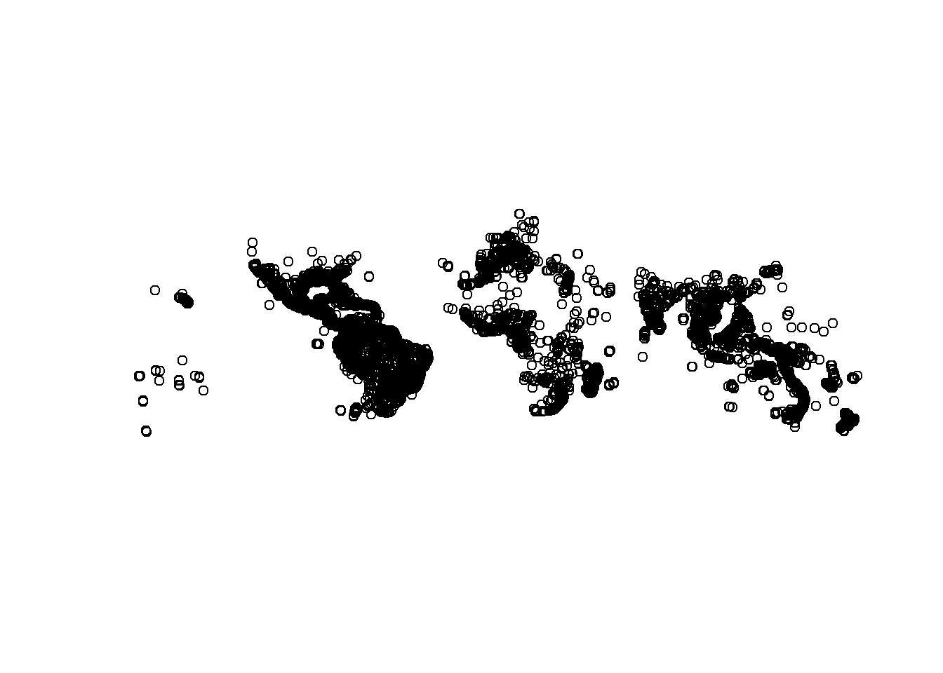
This plots only the geometry. It is useful for a first visual check: do the points appear in plausible parts of the world? You can also plot an attribute:
2.8.4.1 Country polygons with the rnaturalearth package
Occurrence points are easier to interpret when we draw them on top of a base map. We can use rnaturalearth to get country polygons from Natural Earth using function ne_countries().
# First, load the libraries
library(rnaturalearth)
library(rnaturalearthdata)

# Extract a world map from Natural Earth as
# an sf object and select only some important columns
world <- ne_countries(returnclass = "sf") %>%
  select(name_long,
         continent,
         region_un,
         subregion,
         geometry)

# Inspect the object
class(world)
## [1] "sf" "data.frame"## Coordinate Reference System:
## User input: WGS 84
## wkt:
## GEOGCRS["WGS 84",
## DATUM["World Geodetic System 1984",
## ELLIPSOID["WGS 84",6378137,298.257223563,
## LENGTHUNIT["metre",1]]],
## PRIMEM["Greenwich",0,
## ANGLEUNIT["degree",0.0174532925199433]],
## CS[ellipsoidal,2],
## AXIS["latitude",north,
## ORDER[1],
## ANGLEUNIT["degree",0.0174532925199433]],
## AXIS["longitude",east,
## ORDER[2],
## ANGLEUNIT["degree",0.0174532925199433]],
## ID["EPSG",4326]]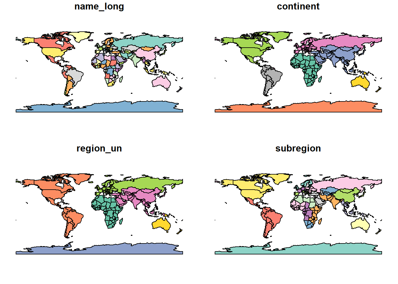
The world object is a polygon layer. Each row represents a country or territory, and the geometry column stores the shape of that country. Some countries, such as Indonesia or the Philippines, contain many islands. These are often stored as multipolygons: many polygon parts belonging to one row.
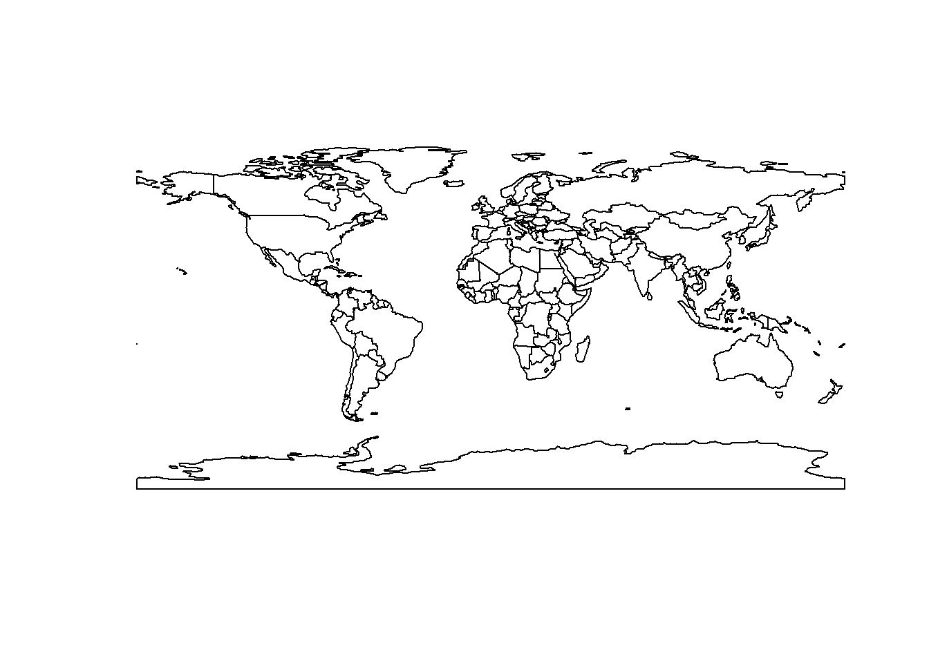
Now we can plot the palm occurrences over our world polygon. We do this by using add = TRUE in the second plot() call, which tells R to add the palm points to the map that is already displayed in the Plots panel, instead of creating a new plot:
# First, plot the world polygon
plot(st_geometry(world), col = "grey60", border = "white")

# Then plot the palm_sf object on top (add = TRUE)
plot(st_geometry(palm_sf), add = TRUE, pch = 16, cex = 0.2)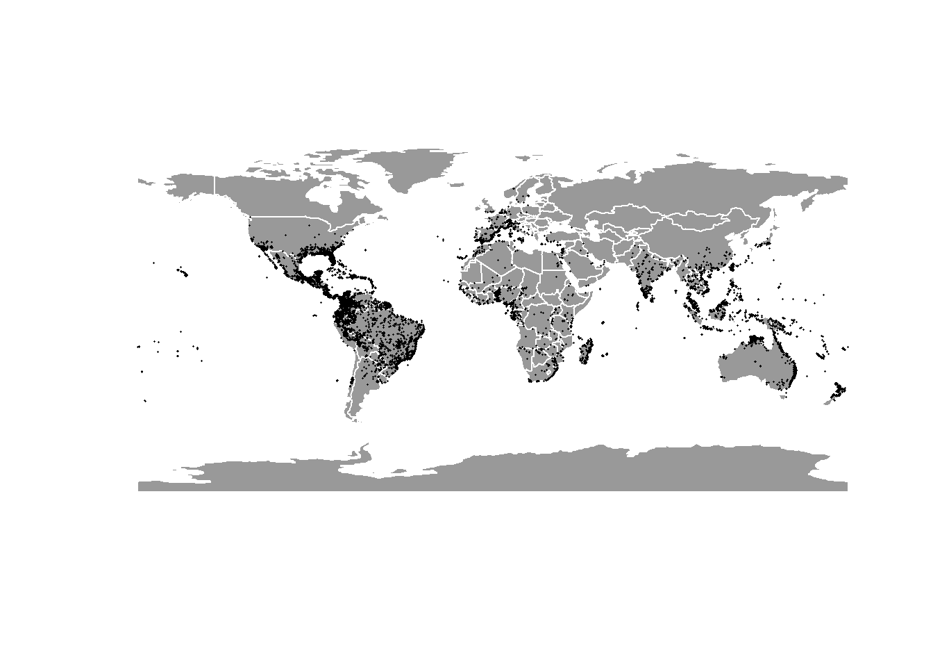
Wow, this already looks very good!
We can also focus on one region, using ne_countries() to extract a polygon for a specific country in the world. Let’s plot Madagascar and its palm occurrences:
# Get country polygon for Madagascar and select only important columns
madagascar <- ne_countries(
  country = "Madagascar",
  returnclass = "sf") %>%
  select(name_long, continent, geometry)

# Plot the madagascar polygon
plot(st_geometry(madagascar), col = "grey60", border = "white")

# Then, plot only the Malagasy occurrences over the polygon
palm_sf %>%
  filter(country == "Madagascar") %>%
  st_geometry() %>%
  plot(add = TRUE)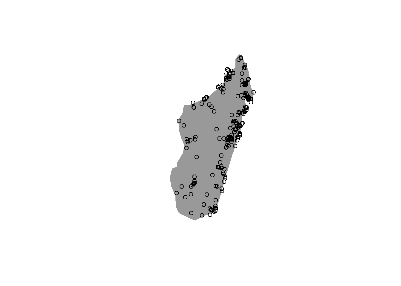
2.8.5 Mapping with ggplot2 and geom_sf()
Because you already know ggplot2, we can use the same plotting logic with spatial objects. The special geom for sf objects is geom_sf(). Here it is important to write data = inside each geom_sf() layer, because we are plotting two different spatial objects in the same figure.
ggplot() +
  geom_sf(data = world, fill = "grey60", color = "white") +
  geom_sf(data = palm_sf, size = 0.5, alpha = 0.3) +
  theme_minimal()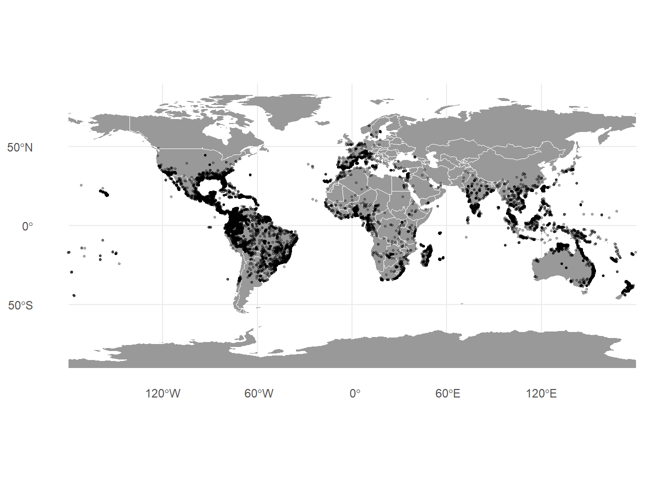
The first layer uses world, which contains the country polygons. This creates the background map. The second layer uses palm_sf, which contains the palm occurrence points. This adds the palm records on top of the world map. Remember that the order of layers is important in ggplot2: layers are drawn one after another, from top to bottom. If we plotted the points first and then added the world polygons, the polygons would cover the points, making the palm records difficult or impossible to see.
With the other geoms from ggplot2 we saw in the previous session, you often write aes(x = ..., y = ...). With geom_sf(), you usually do not need to specify x and y, because the geometry column already contains the spatial coordinates. geom_sf() reads the geometry directly.
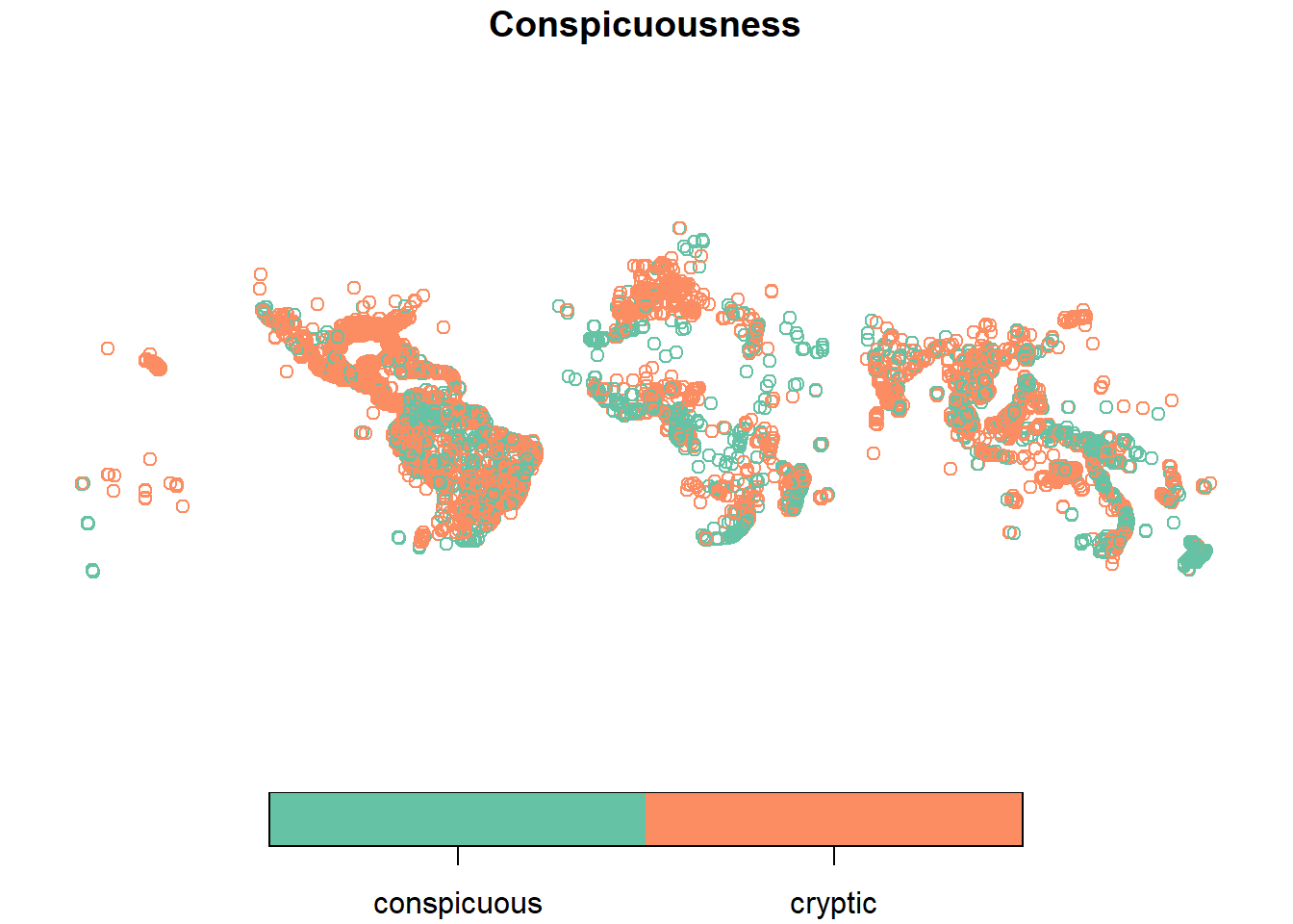
We can also color records by an atribute, such as fruit conspicuousness:
ggplot() +
  geom_sf(data = world, fill = "grey60", color = "white") +
  geom_sf(data = palm_sf, aes(color = Conspicuousness),
    size = 1.5,
    alpha = 0.4) +
  theme_minimal()
Here, two different colors are assigned automatically because Conspicuousness is a categorical variable. If we would plot AverageFruitLength_cm instead, we need a sequential color palette, because fruit length is a continuous variable. ggplot2 is able to automatically recognize if the data is categorical or continuous and can assign a palette accordingly:
ggplot() +
  geom_sf(data = world, fill = "grey60", color = "white") +
  geom_sf(data = palm_sf, aes(color = AverageFruitLength_cm),
          size = 1.5,
          alpha = 0.4) +
theme_minimal() 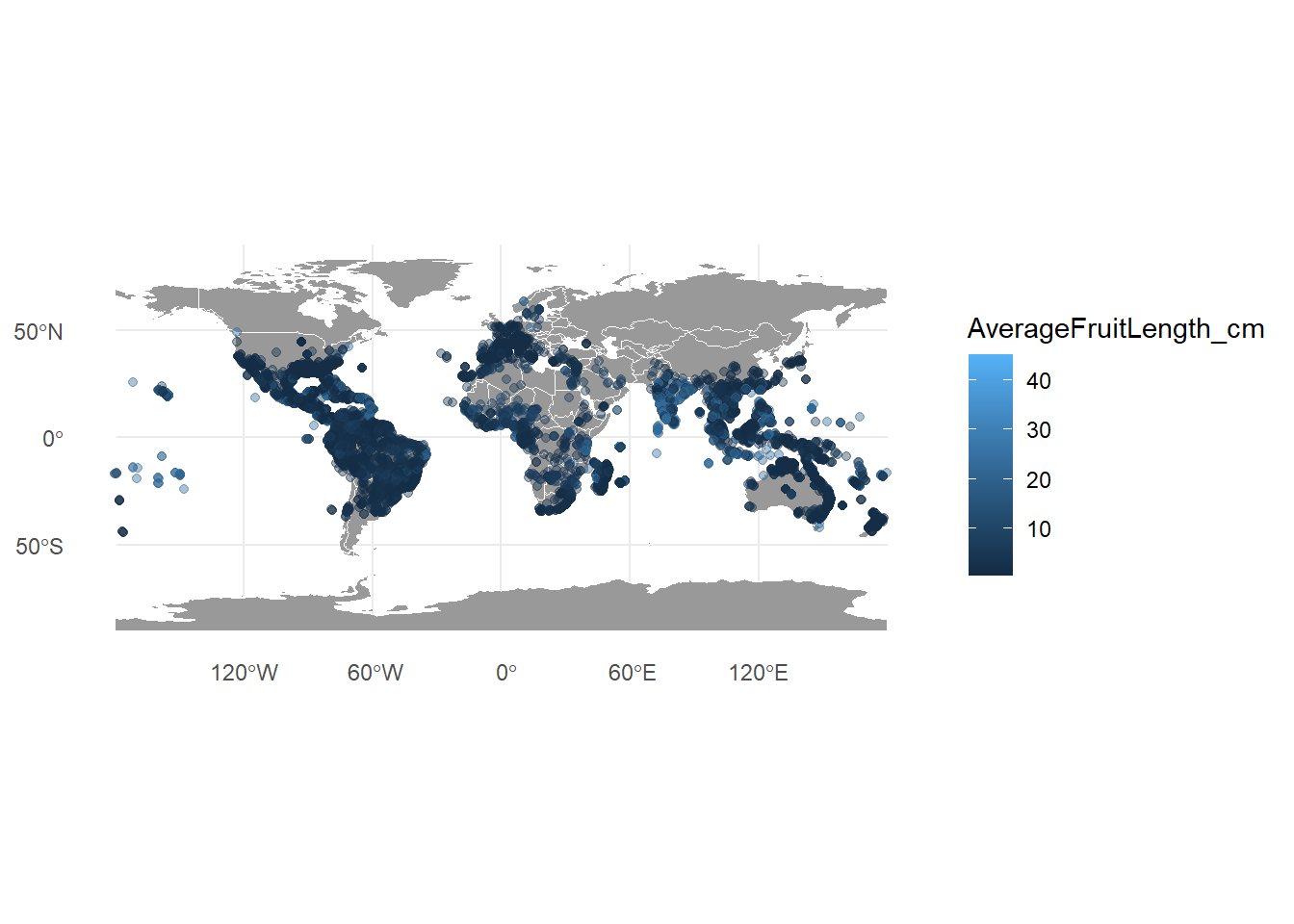
2.8.6 Coordinate Reference Systems and projections
We already explained what is a CRS and how to check it and use it when creating an sf object. Let’s explore this a bit more. Check the CRS of the palm records:
## Coordinate Reference System:
##   User input: EPSG:4326
##   wkt:
## GEOGCRS["WGS 84",
##     ENSEMBLE["World Geodetic System 1984 ensemble",
##         MEMBER["World Geodetic System 1984 (Transit)"],
##         MEMBER["World Geodetic System 1984 (G730)"],
##         MEMBER["World Geodetic System 1984 (G873)"],
##         MEMBER["World Geodetic System 1984 (G1150)"],
##         MEMBER["World Geodetic System 1984 (G1674)"],
##         MEMBER["World Geodetic System 1984 (G1762)"],
##         MEMBER["World Geodetic System 1984 (G2139)"],
##         MEMBER["World Geodetic System 1984 (G2296)"],
##         ELLIPSOID["WGS 84",6378137,298.257223563,
##             LENGTHUNIT["metre",1]],
##         ENSEMBLEACCURACY[2.0]],
##     PRIMEM["Greenwich",0,
##         ANGLEUNIT["degree",0.0174532925199433]],
##     CS[ellipsoidal,2],
##         AXIS["geodetic latitude (Lat)",north,
##             ORDER[1],
##             ANGLEUNIT["degree",0.0174532925199433]],
##         AXIS["geodetic longitude (Lon)",east,
##             ORDER[2],
##             ANGLEUNIT["degree",0.0174532925199433]],
##     USAGE[
##         SCOPE["Horizontal component of 3D system."],
##         AREA["World."],
##         BBOX[-90,-180,90,180]],
##     ID["EPSG",4326]]
As we saw before, this tells us that the palm records use EPSG:4326, also called WGS84. This is a geographic CRS with coordinates measured in degrees of longitude and latitude.
2.8.6.1 Geographic CRS vs projected CRS
A geographic CRS uses angular units, usually degrees. It is good for storing global positions and sharing occurrence records. However, degrees are not equal distances everywhere. One degree of longitude covers a much shorter distance near the poles than at the equator.
A projected CRS represents the curved Earth on a flat surface, usually with coordinates in metres. Projected CRS are better for measuring distances, areas, and creating equal-area grids. However, all map projections distort something: area, shape, distance, direction, or some compromise among them.
Projection choice can strongly affect ecological interpretation. If you compare species richness across grid cells, but the grid cells are not equal in area, tropical and high-latitude regions may not be comparable. If you calculate distances in longitude/latitude degrees as if they were metres, the result will be wrong.
For global biodiversity comparisons, equal-area projections are often preferred when area matters.
Transform the world and palm records to a projected CRS, such as the Equal Earth Greenwich (EPSG:8857), using the function st_transform():
Then, plot the transformed data:
ggplot() +
  geom_sf(data = world_equal_area, fill = "grey60", color = "white") +
  geom_sf(data = palms_equal_area, size = 0.2, alpha = 0.3) +
  theme_minimal() +
  labs(title = "Palm records in an equal-area projection")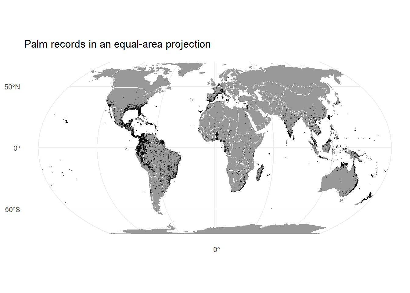
Important: st_transform() is not the same as assigning a CRS
st_transform() changes coordinates from one CRS to another. It should only be used when the object already has the correct CRS assigned.
If an object has no CRS but you know what CRS its coordinates are in, you can assign it with st_set_crs(). If an object already has coordinates in one CRS and you want to convert them to another, then use st_transform().
In most biodiversity occurrence datasets with longitude and latitude, the CRS is usually WGS84 (EPSG:4326), but you should always check the metadata.
A quick summary of different projections, their types, properties, and suitability can be found here.
2.8.7 Reading polygon data from a shapefile
A shapefile is a common spatial vector format. Despite the name, a shapefile is usually not a single file. It is a group of files that must stay together. Typical components are:
- .shp: feature geometry.
- .dbf: attribute table.
- .shx: spatial index.
- .prj: projection information.
If one part is missing, the shapefile may not read correctly or may lose important CRS information.
We will be using the Ecoregions2017 shapefile, which includes information on realms, biomes and ecoregions of Earth as defined by Olson et al. 2001. You can download this from ILIAS and put it in your data folder. It is a zipped (compressed) folder called Ecoregions2017 containing 4 files. First unzip it. Then you can read the files with function st_read(), and inspect it:
## Reading layer `Ecoregions2017' from data source
##   `C:\Users\ploti\Dropbox\Work\Teaching\02_Biodiversity of plants\R_exercise\bsc-biodiv-der-pflanzen\data\Ecoregions2017\Ecoregions2017.shp'
##   using driver `ESRI Shapefile'
## Simple feature collection with 847 features and 15 fields
## Geometry type: MULTIPOLYGON
## Dimension:     XY
## Bounding box:  xmin: -180 ymin: -89.89197 xmax: 180 ymax: 83.62313
## Geodetic CRS: WGS 84## [1] "OBJECTID" "ECO_NAME" "BIOME_NUM" "BIOME_NAME" "REALM"
## [6] "ECO_BIOME_" "NNH" "ECO_ID" "SHAPE_LENG" "SHAPE_AREA"
## [11] "NNH_NAME" "COLOR" "COLOR_BIO" "COLOR_NNH" "LICENSE"
## [16] "geometry"## Coordinate Reference System:
## User input: WGS 84
## wkt:
## GEOGCRS["WGS 84",
## DATUM["World Geodetic System 1984",
## ELLIPSOID["WGS 84",6378137,298.257223563,
## LENGTHUNIT["metre",1]]],
## PRIMEM["Greenwich",0,
## ANGLEUNIT["degree",0.0174532925199433]],
## CS[ellipsoidal,2],
## AXIS["latitude",north,
## ORDER[1],
## ANGLEUNIT["degree",0.0174532925199433]],
## AXIS["longitude",east,
## ORDER[2],
## ANGLEUNIT["degree",0.0174532925199433]],
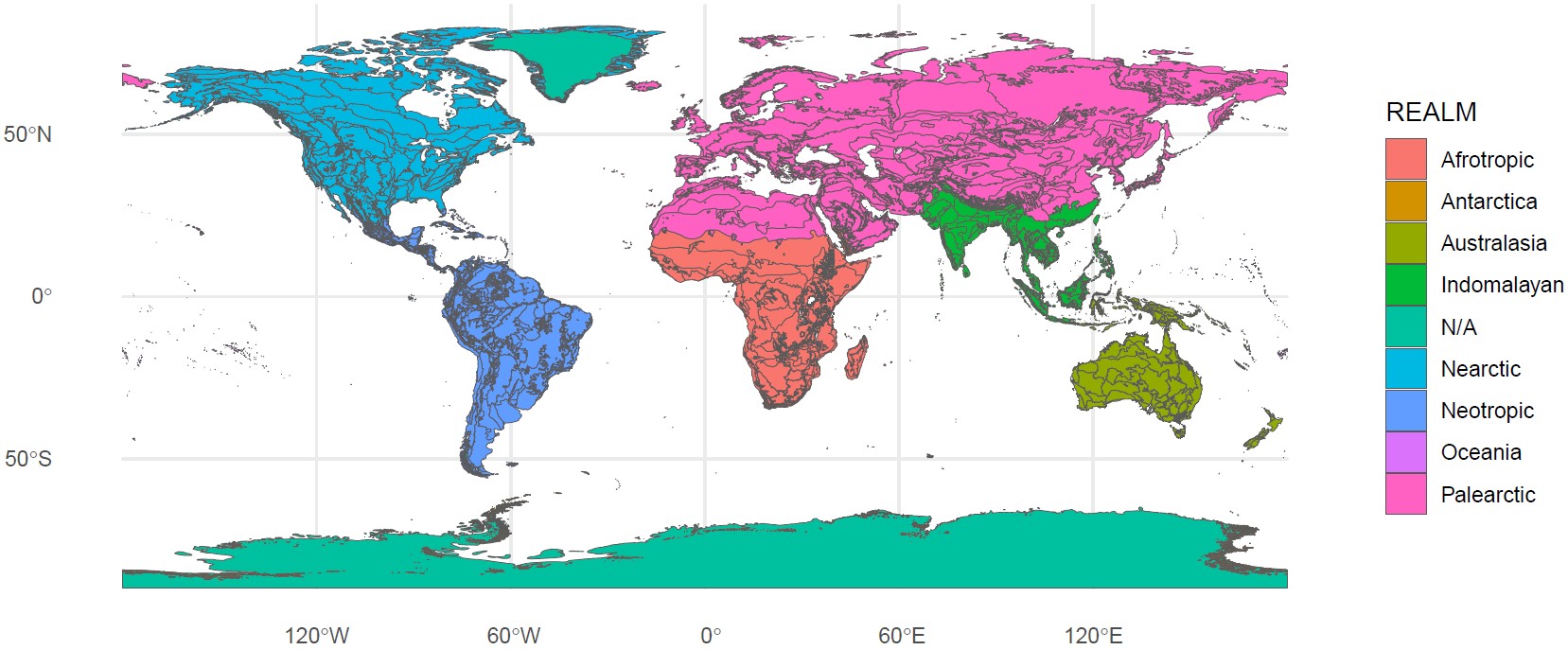
## ID["EPSG",4326]]You can see that it already has the same CRS as our palm data (WGS84). Since this shape file is very large and contains loads of information, do not try to plot it with the plot() function! Or try it, and you will see how long it takes! For example, let’s color the map by the 9 different Realms:
2.8.8 Extract biome information for each palm record
In which biome does each palm record fall? This can be done with a spatial join using function st_join(). A spatial join transfers attributes from one spatial layer to another based on their spatial relationship, similarly to left_join() we used in the last session to join two dataframes by a specific column.
Although both layers use the same CRS, spatial operations can still fail if polygon geometries are invalid. Large global shapefiles sometimes contain small errors such as duplicate vertices, self-intersections, or broken polygon rings. We can often repair these problems with st_make_valid() before using st_join().
# Repair possible errors
biomes_valid <- biomes %>%
  st_make_valid()

# Join to the biomes sf object.
## This might take a while!!!
palm_biomes <- palm_sf %>%
  st_join(biomes_valid)
For each palm point, st_join() looked for the biome polygon containing or intersecting that point. It then copied the biome attributes, such as biome name, into the palm record table. The result palm_biomes is still an sf object, but now each palm record has extra information from the biome map.
We can now count records per biome. When we only want a normal table summary, such as counts per biome, we can remove the geometry temporarily using st_drop_geometry(), which makes the object behave like a normal data frame again. It is often helpful before using count(), group_by(), or summarise().
##                                                  BIOME_NAME     n
## 1            Tropical & Subtropical Moist Broadleaf Forests 37442
## 2  Tropical & Subtropical Grasslands, Savannas & Shrublands  2812
## 3                       Temperate Broadleaf & Mixed Forests  1764
## 4              Tropical & Subtropical Dry Broadleaf Forests  1479
## 5                  Mediterranean Forests, Woodlands & Scrub  1465
## 6               Temperate Grasslands, Savannas & Shrublands  1367
## 7                                                      <NA>  1301
## 8                                                 Mangroves   733
## 9                                Deserts & Xeric Shrublands   703
## 10                                Temperate Conifer Forests   385
## 11                            Flooded Grasslands & Savannas   366
## 12                Tropical & Subtropical Coniferous Forests   129
## 13                          Montane Grasslands & Shrublands    53
## 14                                     Boreal Forests/Taiga     1
Important caveat: If a point lies near a biome boundary, the assigned biome may depend on the spatial resolution and accuracy of both datasets. Occurrence coordinates may be imprecise, and biome boundaries are generalized. For very precise ecological questions, biome data extracted in this way should be treated carefully. That’s why there are also NAs for the biome type, since some points are probably falling outside of the biome boundaries.
Let’s visualize these counts with a barplot:
# First make a dataframe with how many coordinates we have per biome
biome_counts <- palm_biomes %>%
  st_drop_geometry() %>%
  filter(!is.na(BIOME_NAME)) %>%
  count(BIOME_NAME, sort = TRUE)

# Look at the result, the counts are in the column "n"
biome_counts
## BIOME_NAME n
## 1 Tropical & Subtropical Moist Broadleaf Forests 37442
## 2 Tropical & Subtropical Grasslands, Savannas & Shrublands 2812
## 3 Temperate Broadleaf & Mixed Forests 1764
## 4 Tropical & Subtropical Dry Broadleaf Forests 1479
## 5 Mediterranean Forests, Woodlands & Scrub 1465
## 6 Temperate Grasslands, Savannas & Shrublands 1367
## 7 Mangroves 733
## 8 Deserts & Xeric Shrublands 703
## 9 Temperate Conifer Forests 385
## 10 Flooded Grasslands & Savannas 366
## 11 Tropical & Subtropical Coniferous Forests 129
## 12 Montane Grasslands & Shrublands 53
## 13 Boreal Forests/Taiga 1# Now plot the barplot using "n" as the y axes, and reordering
# the biomes in descending order with reorder()
ggplot(biome_counts, aes(x = reorder(BIOME_NAME, n), y = n)) +
geom_col(fill = "plum4") +
coord_flip() +
theme_minimal() +
labs(x = "Biome",
y = "Number of palm records")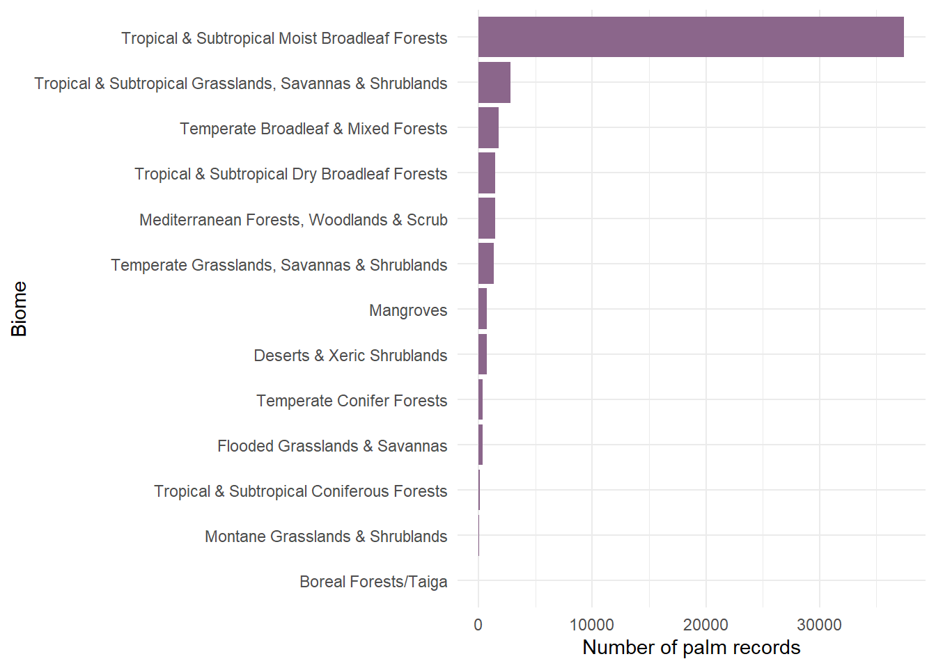
Let’s now map the palm records colored by the five biomes with most palm records:
# First select the five biomes with most palm occurrences
top_biomes <- palm_biomes %>%
  st_drop_geometry() %>%
  count(BIOME_NAME, sort = TRUE) %>%
  filter(!is.na(BIOME_NAME)) %>%
  slice_max(n, n = 5) %>%
  pull(BIOME_NAME)

# Then select only the palm occurrences from the top five biomes
palm_top_biomes <- palm_biomes %>%
  filter(BIOME_NAME %in% top_biomes)

# Plot the palm occurrences colored by biome using the world polygon
# as the background map
ggplot() +
  geom_sf(data = world, fill = "grey60", color = "white") +
  geom_sf(
    data = palm_top_biomes,
    aes(color = BIOME_NAME),
    size = 1.5,
    alpha = 0.5) +
  theme_minimal() +
  theme(legend.position = "bottom") +
  guides(color = guide_legend(nrow = 3)) + # show the legend in 3 rows
  labs(title = "Palm records in the five most common biomes",
       color = "Biome")
2.8.9 Save your map as an image or PDF
After creating your map, you may want to save it for your report or presentation. To save the last plot you created:
2.8.10 Introduction to raster data
As we said before, raster data divide the world into a regular grid of cells or pixels. Each cell stores a value. For example, a raster cell could contain elevation, temperature, precipitation, land cover, or human population density. Many environmental datasets used in ecology are raster datasets.
In this example, we will use annual precipitation (in millimetres) from WorldClim. WorldClim provides global gridded climate data, and its bioclimatic variables are derived from monthly temperature and rainfall values to produce biologically meaningful summaries. For this session we will only look at Madagascar. BIO12 represents annual precipitation, you can download it from ILIAS.
First, install and load the package terra, which is commonly used for raster data in R. Then, read the raster file BIO12.asc with function rast().
# Load the terra package
library("terra")
# Read the raster file with function rast()
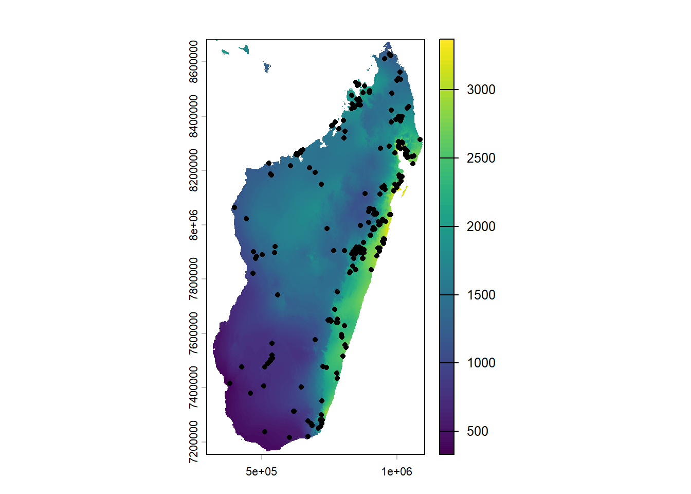
bio12 <- rast("data/BIO12.asc")
# Plot the raster
plot(bio12)
## class       : SpatRaster
## size        : 1528, 803, 1  (nrow, ncol, nlyr)
## resolution  : 1000, 1000  (x, y)
## extent      : 298000, 1101000, 7155000, 8683000  (xmin, xmax, ymin, ymax)
## coord. ref. :
## source      : BIO12.asc
## name        : BIO12
This output tells us that BIO12 is an object of SpatRaster class, the raster object format used by the terra package. The raster has 1528 rows, 803 columns, and 1 layer. This means it is a single-variable raster: each grid cell contains one value, annual precipitation. The resolution is 1000 × 1000, meaning that each raster cell represents an area of 1 km by 1 km. The extent gives the spatial limits of the raster: the minimum and maximum x and y coordinates covered by the file. In this case, the coordinates are not longitude and latitude values, but projected coordinates in meters. The CRS is not shown in the output, so we should check whether it is missing and, if necessary, assign the correct CRS before using the raster together with other spatial data. For the terra package the function is crs():
## [1] ""The crs is indeed missing. From the raster extent and resolution we can see that the coordinates are projected coordinates in metres, not longitude and latitude. Anyway, we know that the projection is WGS84 / UTM zone 38S, with EPSG code 32738, so we can assign it manually:
This step is important because R needs to know the CRS before we can correctly combine the raster with other spatial data, such as palm occurrence points. Since our palm points are in longitude/latitude (EPSG:4326), we should transform them to the raster CRS before extracting precipitation values. We can use st_transform():
# First select only palms from Madagascar
palm_MAD <- palm_sf %>%
  filter(country == "Madagascar")

# Then reproject the Malgasy palms to he raster's CRS
palm_utm <- st_transform(palm_MAD, crs(bio12))
Now we can check if it worked, by plotting the palm points over the raster:
2.8.10.1 Extract raster values
Now we can extract the precipitation value for each palm occurrence. This means that each palm point receives the annual precipitation value of the raster cell in which it falls. We use function extract() from the terra package.
##   ID BIO12
## 1  1  1808
## 2  2  2399
## 3  3  1802
## 4  4  1988
## 5  5  1224
## 6  6  1742
The first column is an ID that matches the order of palm_utm, and the second column contains the extracted precipitation value from BIO12. We can add this value back to palm_MAD:
Now we can plot the palm occurrence records on top of the madagascar map from rnaturalearth, with the points colored by the extracted annual precipitation values:
ggplot() +
  geom_sf(data = madagascar, fill = "grey80", color = "white") +
  geom_sf(
    data = palm_climate,
    aes(color = annual_precip_mm),
    size = 1.5,
    alpha = 0.8) +
  scale_color_viridis_c() +
  theme_minimal() +
  labs(title = "Annual precipitation at palm occurrence records in Madagascar",
    color = "Annual precipitation (mm)") ## Adds a manual title for the legend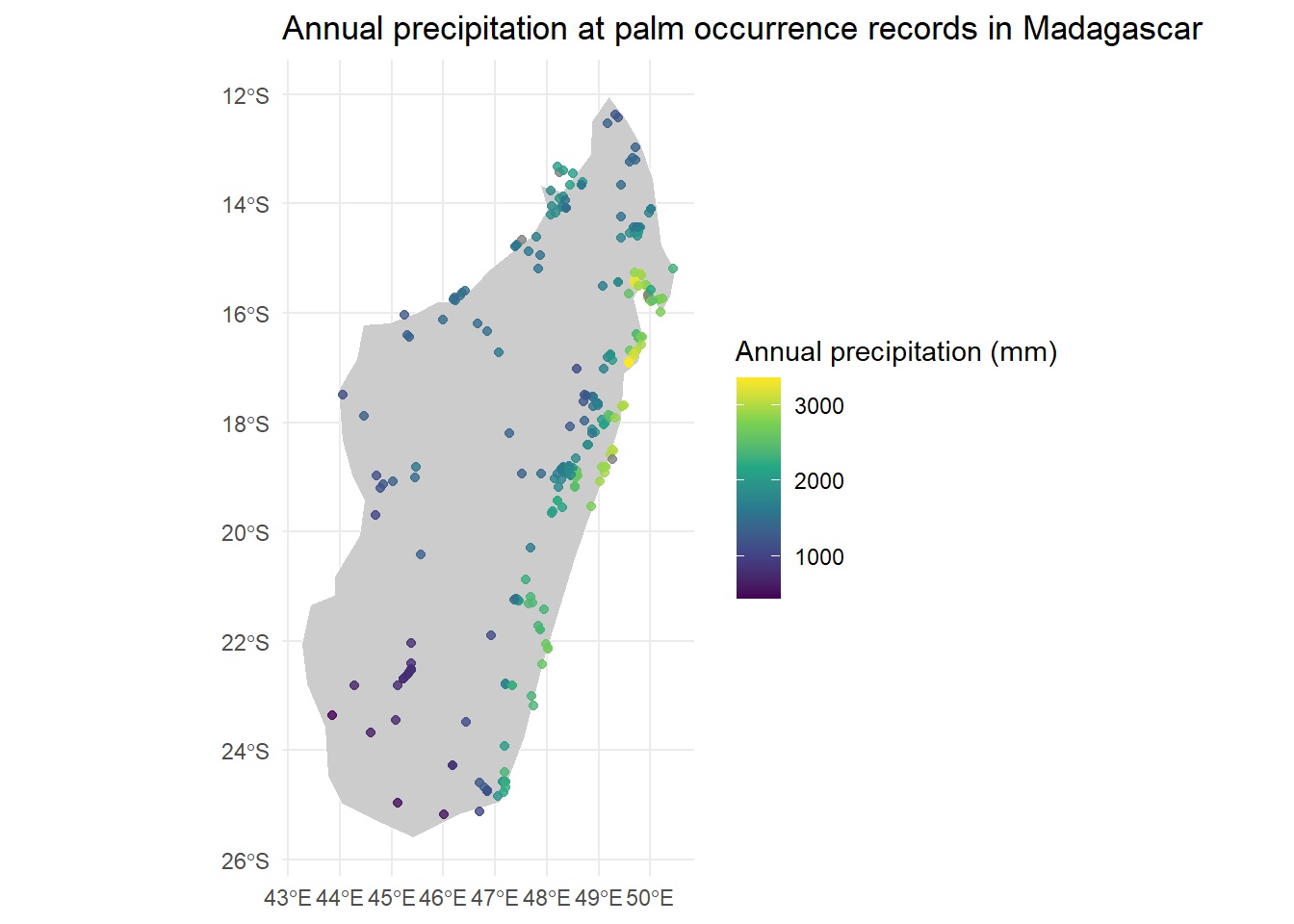
2.8.11 Tasks
Where do we find large, medium and small fruited palms? Using
palm_biomes, create a newsfobject calledpalm_sf_fruitwith a new column called “fruit_size_class” and classify palm records into three fruit-size categories based onAverageFruitLength_cm: small-fruits: fruits ≤ 1 cm; medium-fruits: fruits > 1 cm and < 4 cm; large-fruits: fruits ≥ 4 cm. Then plot palm occurrences worldwide, colored by “fruit_size_class” and useworldas a background map.Using
palm_sf, choose a country of your choice and get thesfobject usingne_countries(). Then spatially filter the palm records so that only records inside that country remain. Create a map with the country polygon in the background and palm occurrences on top. Color the points byMaxStemHeight_musing the viridis color palette for continuous data. Add a legend title.Go to Worldclim, download the worldwide raster map for elevation (elev 10m), put it in your
datafolder and unzip it. This is a layer calledwc2.1_10m_elev.tif. Read it in R, inspect it and plot it. What is its CRS?Plot the
palm_biomesobject over the raster. Extract elevation values for each palm occurrence and join them again topalm_biomes. Can you identify the palm species occurring at the highest altitude, and in which biome? Functionslice_max()from the packagedplyrcan help.