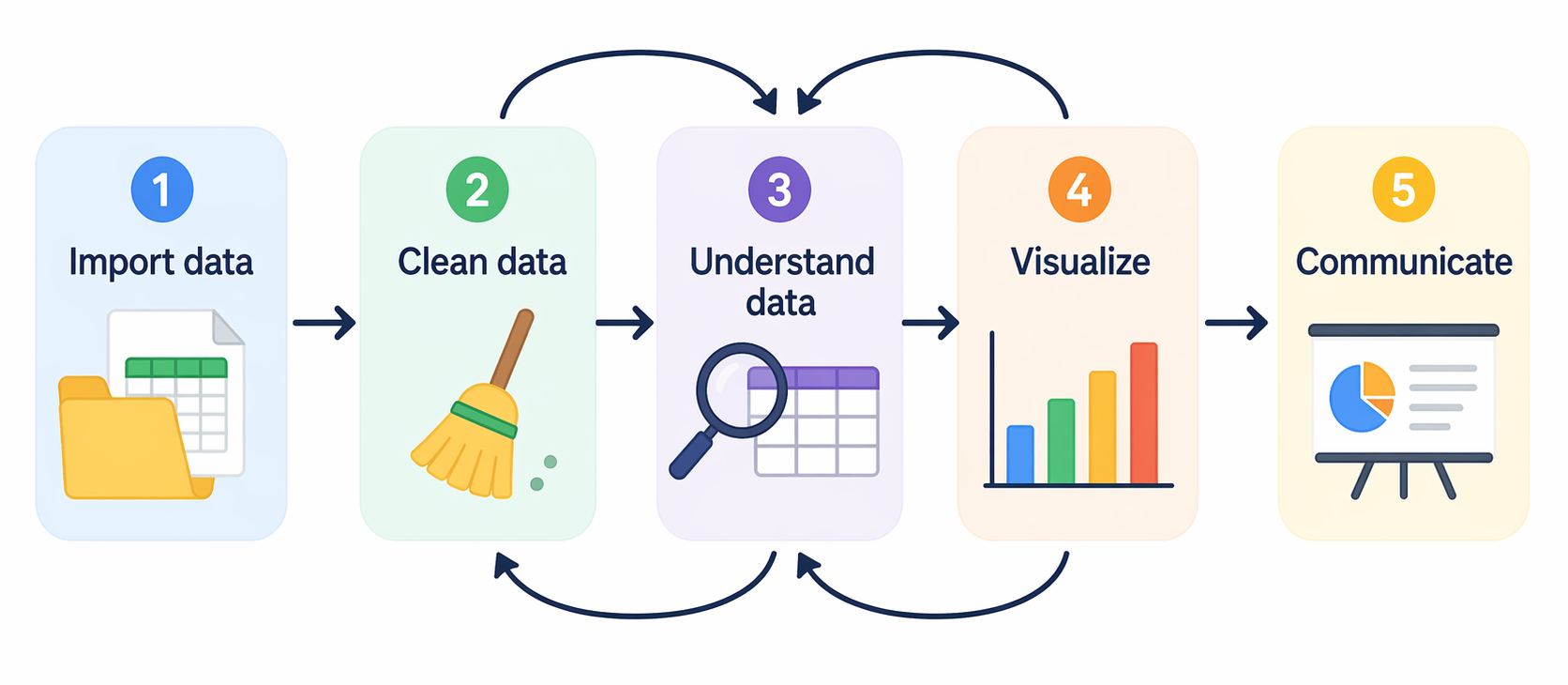
2.6 Cleaning and exploring collection data in R (tidyverse)
2.6.1 Background
In the previous exercise, you learned the basics of working with R. You practiced setting a working directory, creating objects, importing .csv files, inspecting dataframes subsetting data, finding unique values, doing simple summaries, and saving results as .csv files.
In this exercise, we will continue with the same basic ideas, but we will use the tidyverse. The tidyverse is a collection of R packages designed for data science. Its packages share a common grammar, structure, and style, which makes code easier to read, write, and reuse.
Let’s go!
2.6.2 Learning objectives
By the end of this session, you will be able to:
- Understand what the tidyverse is and why it is useful for reproducible data analysis.
- Clean and explore biological collection data using tidyverse functions.
- Use a cleaned occurrence data set to answer simple biodiversity questions independently.
2.6.3 Literature
Wickham H, Cetinkaya-Rundel M & Grolemund G (2023). R for Data Science. Chapter 3: https://r4ds.hadley.nz/data-transform.html
2.6.5 What is the tidyverse?
The tidyverse is a collection of R packages designed for data science.
Some of the packages it includes are:
dplyr: data cleaning and manipulationtidyr: reshaping dataggplot2: plottingreadr: reading and writing tables
Usually, we load all of them together:
Today we will focus mainly on dplyr, one of the core tidyverse packages. dplyr provides a set of simple “verbs” for common data manipulation tasks, such as select() to choose columns, filter() to choose rows, mutate() to create new columns, summarise() to calculate summaries, etc. The syntax is generally as follows:
The first argument is most times a data frame.
The subsequent arguments typically describe which columns to operate on using the variable names (without quotes).
The output is always a new data frame.
The same tasks can often be done in base R, but tidyverse code is usually more consistent and easier to read, especially when several steps are combined. For example, instead of writing many separate commands or nested functions, we can use the pipe operator %>% to build a clear workflow from top to bottom, as we will see later.
Let’s start with opening your project and creating a new R script for today’s R exercise (for example 06_tidyverse.R).
2.6.6 Our dataset: GBIF palm records
In this tutorial, we will work with GBIF occurrence records for the palm family, Arecaceae. Download the data for this session from ILIAS and put it in your data folder. Then import the file into R:
# We could check the structure of the data with base R as you already learnt:
str(palms_raw)

# Or we can use glimpse() from tidyverse:
glimpse(palms_raw)
In R data frames, you often see short type labels before each column name, like <dbl>, <chr>, <int>, and so on:
| Type label | Full meaning | What it stores | Example |
|---|---|---|---|
<dbl> |
double | Decimal numbers, and often general numeric values | 3.14, 10, 2.5 |
<int> |
integer | Whole numbers | 1, 25, 100 |
<chr> |
character | Text / strings | "hello", "Berlin" |
<lgl> |
logical | Boolean values | TRUE, FALSE, NA |
<fct> |
factor | Categorical values with fixed levels | "low", "medium", "high" |
<num> |
numeric | General numeric type, usually similar to double | 42, 3.5 |
<date> |
Date | Calendar dates | 2026-04-24 |
<dttm> |
date-time | Date plus time | 2026-04-24 14:30:00 |
<list> |
list-column | Complex objects inside cells | vectors, models, nested data |
Knowing the data type is important because it tells R what kind of information is stored in each column and therefore what operations are possible. For example, a column with type <dbl> or <int> is treated as a number, so R can calculate things like the mean, sum, minimum, maximum, etc. But a column with type <chr> is treated as text, so R cannot calculate an average from it, even if the values look like numbers.
## [1] 1953744778## Warning in mean.default(palms_raw$kingdom): argument is not numeric or logical:
## returning NA## [1] NA## [1] 2007.347## [1] NA## [1] 111982.6.7 The pipe: %>%
One of the most important tidyverse tools is the pipe. It means: “Take the result from the left side and send it into the next function”
The pipe becomes useful when we want to do several steps. For example, if we would want to know how many unique countries we have data for:
# In base R we would write:
length(unique(palms_raw$country))

# With the pipe:
palms_raw$country %>%
  unique() %>%
  length()

# Sort the unique countries alphabetically:
palms_raw$country %>%
  unique() %>%
  sort()

# Look at the 10 top countries with most occurrences:
palms_raw$country %>%
  table() %>%
  sort(decreasing = TRUE) %>%
  head(10)

# Instead of:
head(sort(table(palms_raw$country), decreasing = TRUE), 10)
You can write the pipe faster in R with the shortcut Ctrl + Shift + M (Windows) or Cmd + Shift + M (Mac).
2.6.8 Selecting columns
It’s not uncommon to get data sets with hundreds of variables (columns). In this situation, the first challenge is often just focusing on the variables you’re interested in. select() allows you to rapidly zoom in on a useful subset using operations based on the names of the variables:
# Keep the most important variables for the next cleaning steps:
palms_small <- palms_raw %>%
  select(
    family,
    genus,
    species,
    decimalLongitude,
    decimalLatitude,
    country,
    locality,
    stateProvince,
    year,
    basisOfRecord)
Look at the new dataset:
You can also use select() to rename columns at the same time than selecting them, suing the syntax: new_name = old_name.
2.6.9 Counting records in categories
When working with biodiversity data, we often want to know how records are distributed across different categories. For example, we may want to know which countries have the most records, which species are most frequently collected, or which genera are best represented in a data set. The count() function is useful because it quickly counts how many rows belong to each group. For example:
# How many records per country?
palms_small %>%
  count(country)

# Sort from most records to fewest and show the first 10:
palms_small %>%
  count(country, sort = TRUE) %>%
  head(10)

# Sort from most records to fewest and show the last 10:
palms_small %>%
  count(country, sort = TRUE) %>%
  tail(10)

# Which kind of observations do we have in or data and how many of each?
palms_small %>%
  count(basisOfRecord, sort = TRUE)

# Count how many records there are for each species in each country,
# then sort them from highest to lowest and show the first 30:
palms_small %>%
  count(country, species, sort = TRUE) %>%
  head(30)
This helps us detect patterns in the data, such as which regions could be hotspots for palms.
2.6.10 Filtering rows
One of the fundamental operations in almost any data analysis is filtering data based on specific conditions. The filter() function in dplyr allows us to extract rows from a data set that meet certain criteria.
# For example, keep only records from Madagascar:
palms_small %>%
  filter(country == "Madagascar") %>%
  glimpse()
Important symbols:
| Symbol | Meaning |
|---|---|
== |
equal to |
!= |
not equal to |
> |
greater than |
< |
less than |
>= |
greater than or equal to |
<= |
less than or equal to |
is.na() |
is missing |
!is.na() |
is not missing |
You can also combine conditions with & or , to indicate “and” (check for both conditions) or with | to indicate “or” (check for either condition):
# Keep records from Madagascar after the year 2000:
palms_small %>%
  filter(country == "Madagascar", year > 2000) %>%
  glimpse()

# Same result using &
palms_small %>%
  filter(country == "Madagascar" & year > 2000) %>%
  glimpse()

# Keep records from Madagascar OR Brazil OR India
palms_small %>%
  filter(
    country == "Madagascar" | country == "Brazil" | country == "India") %>%
  glimpse()

# Same idea, but easier to read
palms_small %>%
  filter(country %in% c("Madagascar", "Brazil", "India")) %>%
  glimpse()

# Records with coordinates
palms_small %>%
  filter(
    !is.na(decimalLongitude),
    !is.na(decimalLatitude)) %>%
  glimpse()

# Records with collection year
palms_small %>%
  filter(!is.na(year)) %>%
  glimpse()

# Records that are a "HUMAN_OBSERVATION", a "PRESERVED_SPECIMEN" or an "OCCURRENCE"
palms_small %>%
  filter(basisOfRecord %in% c(
    "HUMAN_OBSERVATION",
    "PRESERVED_SPECIMEN",
    "OCCURRENCE")) %>%
  glimpse()

# Combine many filtering options: Keep recent records from Madagascar,
# Brazil and India, from the year 2000 and only if they have species name
# and genus name
palms_small %>%
  filter(
    country %in% c("Madagascar", "Brazil", "India"),
    year >= 2000,
    !is.na(species),
    !is.na(genus)) %>%
  glimpse()
2.6.11 Sorting rows
arrange() is used to sort the rows of a data set based on one or more columns. This is useful when we want to see the largest or smallest values first, such as the countries with most records, the oldest collection years, or the species with the highest number of occurrences.
By default, arrange() sorts values from small to large or from A to Z.
# Sort by year from oldest to newest and show the first 6:
palms_small %>%
  arrange(year) %>%
  head()
# The oldest observation is from Chamaerops humilis in France in 1757

# Arrange from newest to oldest using desc():
palms_small %>%
  arrange(desc(year)) %>%
  head()

# Sort by country, and then by year within each country:
palms_small %>%
  arrange(country, year) %>%
  head()
2.6.12 Creating new columns from existing information
mutate() is used to create new columns or modify existing columns in a data set. This is useful when we want to add extra information, simplify values, or create categories that make the data easier to analyse.
For example, we can create a new column “record_period” to classify our records into “old” or “recent”, depending the year they were sampled/observed. We will use the function if_else() which is used to create values based on a condition:
# Classify records collected before the year 2000 as "old",
# and after as "recent"
palms_small <- palms_small %>%
  mutate(
    record_period = if_else(year >= 2000, "recent", "old"))

# Then you can check how many "recent" vs "old" records we have:
palms_small %>%
  count(record_period)
## record_period n
## 1 old 40155
## 2 recent 198647
## 3 <NA> 11198This means: if year is 2000 or later, write “recent”. Otherwise, write “old”. So a record from 2015 becomes “recent”, while a record from 1980 becomes “old”. if_else() only works for two possible categories. To create a column with more than two possible categories, we use case_when(). We could classify the records into 3 categories: “before 1950”, “1950-1999” and “2000 or later”. We also create an explicit category for records with missing years “missing year”.
# The basic structure of case_when():
case_when(
  condition1 ~ value1,
  condition2 ~ value2,
  condition3 ~ value3,
  TRUE ~ default_value)
# Classify records into different time periods:
palms_small <- palms_small %>%
mutate(
record_period = case_when(
is.na(year) ~ "missing year",
year < 1950 ~ "before 1950",
year >= 1950 & year < 2000 ~ "1950-1999",
year >= 2000 ~ "2000 or later"))
# And now check the new classification:
palms_small %>%
count(record_period)## record_period n
## 1 1950-1999 36971
## 2 2000 or later 198647
## 3 before 1950 3184
## 4 missing year 111982.6.13 Summarising data
summarise() is used to calculate summary values from a data set. It creates a new data frame by reducing many rows into one or a few summary results. This is useful when we want to answer questions such as: How many records are there? What is the earliest collection year? What is the latest collection year? How many species are represented?
For example, we can summarise the whole palm dataset:
palms_small %>%
  summarise(
    records = n(), # counts the number of rows
    earliest_year = min(year, na.rm = TRUE), # finds the earliest year
    latest_year = max(year, na.rm = TRUE), # finds the latest year
    number_of_species = n_distinct(species)) # counts the number of unique species
summarise() becomes especially useful together with group_by(). For example, we can calculate summaries for each country:
# Create summary statistics per country, then arrange
# countries with most species to least and show the first 20
palms_small %>%
  group_by(country) %>%
  summarise(
    records = n(),
    species = n_distinct(species),
    earliest_year = min(year, na.rm = TRUE),
    latest_year = max(year, na.rm = TRUE)) %>%
  arrange(desc(species)) %>%
  head(20)
2.6.14 Joining data
In biodiversity research, we often work with different data sets that contain different kinds of information. Therefore, it is important to be able to join those data sets by a specific column where names match. This is what the join functions from the dplyr package allow us to do. They all have the same interface: they take a pair of data frames (x and y) and return a new data frame. The order of the rows and columns in the output is primarily determined by x. The most widely used is left_join(). left_join() keeps all rows from the first data set and adds matching information from the second data set. Let’s look at trait data for our palm species, published in the PalmTraits 1.0 database (Kissling et al. 2019):
# Use read_delim() from the readr package to read the .txt file:
traits <- read_delim("data/PalmTraits_1.0.txt", delim = "\t")

glimpse(traits)
So the column with species names in traits is “SpecName”, while in palms_small was “species”.
# This would join both data sets entirely by species name
palms_small %>%
  left_join(traits, by = c("species" = "SpecName"))
# Let's join the occurrence data set to only one trait:
palms_fruit_length <- palms_small %>%
left_join(
traits %>%
select(SpecName, AverageFruitLength_cm),
by = c("species" = "SpecName")) %>%
glimpse()You can then ask, for example, which species with occurrence records have the largest fruits:
# Top 10 palms with largest fruits in our data base:
palms_fruit_length %>%
  select(species, AverageFruitLength_cm) %>%
  distinct() %>%  # keeps only unique entries
  arrange(desc(AverageFruitLength_cm)) %>%
  head(10)

# Top 10 palms with smallest fruits in our data base:
palms_fruit_length %>%
  select(species, AverageFruitLength_cm) %>%
  filter(!is.na(AverageFruitLength_cm)) %>% # filters out missing data
  distinct() %>%  # keeps only unique entries
  arrange(desc(AverageFruitLength_cm)) %>%
  tail(10)

# How many records have data vs missing data?
palms_fruit_length %>%
  summarise(
    total_records = n(),
    records_with_fruit_length = sum(!is.na(AverageFruitLength_cm)),
    records_without_fruit_length = sum(is.na(AverageFruitLength_cm)))
Let’s visualize 2 simple things using plotting functions from base R:
- Histogram of fruit length
hist(
  palms_fruit_length$AverageFruitLength_cm[!is.na(palms_fruit_length$AverageFruitLength_cm)],
  main = "Distribution of palm fruit length",
  xlab = "Average fruit length (cm)",
  ylab = "Number of records")
- Boxplot of fruit length by record period
boxplot(
  AverageFruitLength_cm ~ record_period,
  data = palms_fruit_length,
  main = "Palm fruit length by record period",
  xlab = "Record period",
  ylab = "Average fruit length (cm)")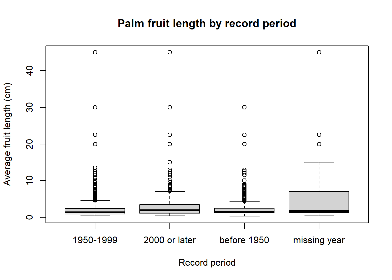
2.6.15 Cleaning biodiversity data
As you have seen, in real biodiversity data, we rarely start with a perfect data set. Collection and occurrence data often contain missing values, old records, incomplete coordinates, different types of records, or taxonomic names that do not match other data sets.
Cleaning means making careful decisions about which records are useful for a specific question. For example, a record without coordinates may still be useful for counting species in a country, but not for mapping distributions. A record without a year may still show that a species was recorded somewhere, but it cannot be used to study changes through time.
Before cleaning, we should ask: What do we want to use this dataset for?
Common problems in biodiversity data include:
- Missing information: species names, coordinates, years, countries, or trait values may be missing.
- Taxonomic problems: species names may be outdated, misspelled, unresolved, or only identified to genus level.
- Geographic problems: coordinates may be missing, imprecise, swapped, outside the correct country, or placed at 0, 0.
- Different record types: herbarium specimens, human observations, living specimens, and general occurrence records may not mean the same thing.
- Sampling bias: records show where species were collected or observed, not necessarily where they truly occur or how common they are.
The most important rule is that cleaning should be transparent and reproducible: someone else should be able to read your methods section and/or code and understand which records were kept, which were removed, and why.
2.6.16 Task
Now it is your turn to combine the functions you have learned.
Create a new dataset called palms_clean, starting from palms_raw. This dataset should contain only the records that are useful for a basic analysis of palm occurrences, and add one trait from the trait dataset:
keep only the columns we need
rename some columns to simpler names
remove records without species names
remove records without collection or observation year
create a new column classifying your dataset into categories of your choice
2.6.16.1 Questions:
- How many records were removed during cleaning?
- How many unique species does your clean dataset contain?
- How many unique countries do you have data for?
- Which species has the most records?
- Which
record_typeis most common in the clean dataset? - Write a short reflection paragraph: What was your attitude towards R before this exercise, how did your attitude change during the exercise, and why? Which code block or function did you find most interesting or most challenging, and why?